Mar
14
Watch Out for Those Splits, from Vic Niederhoffer and Alex Castaldo
March 14, 2013 |
 Written in honour of all splitters, rookies and lookbackers:
A common pursuit in decision making is to compare data of many kinds and find the best way of separating the observations into different classes.
For example you mite be considering what are the factors that contribute to long life. Weight, height, mid range of parents age , % of meat consumed , exercise mite be the variables. You mite find that when parents mid range was above 140, and meat eaten less than 2 times week, and exercise more than 5 hours a day, the longevity is 10 years higher than the average.
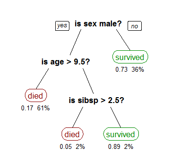
Trees are usually used to separate the groups. An example picture of such a tree is here: [pic ] Lots of good pictures of such trees and a discussion of a typical tree sort is in An Introduction to Classification and Regression Tree (cart) by Roger Lewis. And programs like CART and AID and many modern variants are widely used in medicine and markets. In fact all market people systematically or implicitly consider such problems. When does the market go up? When gold is down more than 10, when bonds are up more than 100, and the previous 5 day sp move is between -1% and 0 %? The problem is that there are many variables to consider, and many levels at which one would reasonably split the data.
A good starting point in considering such problems is to note that when there are two mutually exclusive groups X and Y the variance of the difference between means is the sum of the variances of the means. The variance of a mean is the variance of an individual observation divided by the number of observations. For example, consider the average move in sp during a day has a sd of 10 and variance of 100. If you take two independent samples of 10 from such a distribution , the variance of one mean will be 100/10= 10 and the variance of the difference between means is 20. The standard dev of the difference is 4.4 What does this mean in practice? One will round. A 50% confidence interval in which 50% of the observation range is 0.65 x 4.4 = 3 points on either side of the difference between means which we'll assume to be 0. That means that by chance half of all the observations will show a difference in means ranging from -3 to +3. To find a region where 95% of the observations lie, ie. A 95% confidence interval we'd multiply 2 x 4.4 =8.8. In other words to find a difference that has less than a 5% chance of occurring thru randomness we would have to find a difference between means of 8.8 on any binary split.
But of course that's not all. Normally we look at 2, or 3 or 4 different splits to find the one that gives the greatest difference. It turns out that if we look at the highest of two differences, the average difference is 1.5 times as high as for one difference. In other words by randomness , the standard deviation for the highest of 2 difference between means is 1.5 x 4.4 = 6 a 50% confidence interval assuming randomness for the highest of 2 differences is 0.65 x 6 or from -4 to + 4. A 95% confidence interval would be between 2×6 and -2 x 6 i.e. between -12 and +12.
Now there were several assumptions made in this analysis. We assumed normality. And we didn't take account that there is sampling without replacement for one. And there are two cases: you look at the algebraic difference (2 tailed test, as above) or you try to maximize the *magnitude* of the difference (the 1 tailed approach). To get a good handle on it, Doc and I simulated what would happen if we divided up 20 random observations from a distribution that had a mean of 0 and a standard deviation of 10. This corresponds to the most frequent and typical thing one does when dividing up stock market changes in points (S&P rises or falls by about 10 full points a day). We then took two random subsamples of 10 each and calculated the mean of each of the two groups of 10. We then looked at the absolute value of the average difference between means when we repeated the process 1000 times. It turns out that the average absolute difference between means is 3.5 for a single split (this 3.5 absolute difference is in line with the std dev of 4.4 previously estimated)), 5 for the highest of two splits, and about 6 for the highest of 3 splits. This leads to incredibly high differences that you must be aware of when you split data to have anything more than a 50% chance that the difference occurred thru luck alone. To be 95% sure that you have something departing from luck for the highest of 3 splits you'd need a difference between the groups of 10. As the numbers in the group get less than 10 ,i.e. for a second or third split, the numbers would get increasingly large. This is a warning to all who search for regularities in data using methods that are implicitly or explicitly like tree sorts. By vic and doc.
Here is a more extensive table of simulation results
Table 1
Col A: number of observations being split
Col B: number of splits considered, best one is chosen
——-
Col C: mean absolute difference generated by best split (in S&P points)
Col D: standard deviation of absolute difference
Col E: lower 5% confidence interval
Col F: upper 95% confidence interval
20 1 | 3.56 2.66 0.27 8.65
20 2 | 4.97 2.67 1.24 9.81
20 3 | 5.84 2.64 2.07 10.55
20 4 | 6.45 2.55 2.84 11.05
48 1 | 2.26 1.72 0.18 5.63
48 2 | 3.25 1.71 0.90 6.40
48 3 | 3.75 1.66 1.36 6.78
48 4 | 4.20 1.68 1.79 7.24
Table 2 same as above but
Col C: average (algebraic) difference between means (in S&P points)
Col D: standard deviation of difference between means
20 1 | -0.06 4.61
20 2 | -0.13 5.62
20 3 | 0.01 6.42
20 4 | -0.07 6.88
Let's try to apply this to a typical example.
The 30 year bonds each day have a move of about 80 points.i.e a move from 142 exactly to 142 and 26 /31. Call that the stand dev . Let's say you have 100 observations of bonds in your sample. And you split it into two equal halves based on whether gold is up the previous day or down. The variance of any mean difference would be 6400 x2 /50 =256 . That gives a stand dev of 16.
Turn to the prob that a standard normal deviate will be between -z and + z. the prob is 50% that a normal deviate will be etween -0.65 and + 0.65, the prob is 90% that a stand norm dev will be betweeen -1.6 andd +1.6. Thus if you find a difference that's less than 0.6 x 16 = 10 its 50% chance, and its 90% chance to be 1.6 x 16
Comments
Archives
- June 2026
- May 2026
- April 2026
- March 2026
- February 2026
- January 2026
- December 2025
- November 2025
- October 2025
- September 2025
- August 2025
- July 2025
- June 2025
- May 2025
- April 2025
- March 2025
- February 2025
- January 2025
- December 2024
- November 2024
- October 2024
- September 2024
- August 2024
- July 2024
- June 2024
- May 2024
- April 2024
- March 2024
- February 2024
- January 2024
- December 2023
- November 2023
- October 2023
- September 2023
- August 2023
- July 2023
- June 2023
- May 2023
- April 2023
- March 2023
- February 2023
- January 2023
- December 2022
- November 2022
- October 2022
- September 2022
- August 2022
- July 2022
- June 2022
- May 2022
- April 2022
- March 2022
- February 2022
- January 2022
- December 2021
- November 2021
- October 2021
- September 2021
- August 2021
- July 2021
- June 2021
- May 2021
- April 2021
- March 2021
- February 2021
- January 2021
- December 2020
- November 2020
- October 2020
- September 2020
- August 2020
- July 2020
- June 2020
- May 2020
- April 2020
- March 2020
- February 2020
- January 2020
- December 2019
- November 2019
- October 2019
- September 2019
- August 2019
- July 2019
- June 2019
- May 2019
- April 2019
- March 2019
- February 2019
- January 2019
- December 2018
- November 2018
- October 2018
- September 2018
- August 2018
- July 2018
- June 2018
- May 2018
- April 2018
- March 2018
- February 2018
- January 2018
- December 2017
- November 2017
- October 2017
- September 2017
- August 2017
- July 2017
- June 2017
- May 2017
- April 2017
- March 2017
- February 2017
- January 2017
- December 2016
- November 2016
- October 2016
- September 2016
- August 2016
- July 2016
- June 2016
- May 2016
- April 2016
- March 2016
- February 2016
- January 2016
- December 2015
- November 2015
- October 2015
- September 2015
- August 2015
- July 2015
- June 2015
- May 2015
- April 2015
- March 2015
- February 2015
- January 2015
- December 2014
- November 2014
- October 2014
- September 2014
- August 2014
- July 2014
- June 2014
- May 2014
- April 2014
- March 2014
- February 2014
- January 2014
- December 2013
- November 2013
- October 2013
- September 2013
- August 2013
- July 2013
- June 2013
- May 2013
- April 2013
- March 2013
- February 2013
- January 2013
- December 2012
- November 2012
- October 2012
- September 2012
- August 2012
- July 2012
- June 2012
- May 2012
- April 2012
- March 2012
- February 2012
- January 2012
- December 2011
- November 2011
- October 2011
- September 2011
- August 2011
- July 2011
- June 2011
- May 2011
- April 2011
- March 2011
- February 2011
- January 2011
- December 2010
- November 2010
- October 2010
- September 2010
- August 2010
- July 2010
- June 2010
- May 2010
- April 2010
- March 2010
- February 2010
- January 2010
- December 2009
- November 2009
- October 2009
- September 2009
- August 2009
- July 2009
- June 2009
- May 2009
- April 2009
- March 2009
- February 2009
- January 2009
- December 2008
- November 2008
- October 2008
- September 2008
- August 2008
- July 2008
- June 2008
- May 2008
- April 2008
- March 2008
- February 2008
- January 2008
- December 2007
- November 2007
- October 2007
- September 2007
- August 2007
- July 2007
- June 2007
- May 2007
- April 2007
- March 2007
- February 2007
- January 2007
- December 2006
- November 2006
- October 2006
- September 2006
- August 2006
- Older Archives
Resources & Links
- The Letters Prize
- Pre-2007 Victor Niederhoffer Posts
- Vic’s NYC Junto
- Reading List
- Programming in 60 Seconds
- The Objectivist Center
- Foundation for Economic Education
- Tigerchess
- Dick Sears' G.T. Index
- Pre-2007 Daily Speculations
- Laurel & Vics' Worldly Investor Articles