 |
The Chairman
|
5/7/2005
CUSUM Control Charts
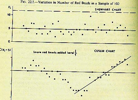
The cumulative sum control chart is a standard quality control chart used to detect changes in the mean output of such things as the output of a machine, the thickness of the asphalt on a road, the amount of bacteria in an infection, the steadiness of heartbeats. It has been used in financial application to study changes in the enthusiasm for IPOs and to detect changes in price.
It turns out that a cumulative sum chart is almost identical to the filter techniques popularized by Alexander and Cootner in the 1960's , a point well covered and analyzed on the SmartQuant site . Acheson Duncan, in his classic work "Qualtity Control and Industrial Statistics," summarizes the advantages of CUSUMs as the "possibility of picking a sudden and persistent change in the process average more rapidly than a comparable (nondynamic Shewhart chart) especially if the change is not large. The key variable in a CUSUM chart is to compare the last point obtained with the lowest (or highest) point previously obtained. Thus, if you go from well below the mean to above or vice versa, the CUSUM is more sensitive than the standards that just look for a breakout from a fixed base. Yes, the CUSUM chart is like a Bollinger Band. The way it's used in practice is to compute the standard deviation from the past observations. Then to note how the current observation compares to the standard, like 0 mean. Next to plot the sum of the amounts above the standard and compare it to a cutoff point, Finally, to use a nomograph to see if the cumulative deviation from the past standard deviation is large enough to give your cutoff point the proper sensitivity without exposing it too much to false alarms.
The process cries out for simulation and direct applications to stock prices. One purpose would be to find out when a trend has been established in the minds of the believers and stoppers with a view to accommodating their visualizations and also finding an early way of detecting a shift in regime in some markets with subsequent testing of whether the subsequent distribution of prices can be forecast. Consider for example, the last 14 changes in S&P futures as of May 6:
+5, -4, -0.5, +9, +3, +5, +15, -14, +4, -10, +7, -4, +22, -16, +9.
Simulating such a process with the artful simulator Mr. Downing (using the last 50 changes) gives us an idea of how much the variation from a low to high, or high to low, might be for the next 1, 2, 5, 10, and 20 days, as follows:
| Days Ahead | Lowest 5% | Highest 5% |
|---|---|---|
| 1 | -16 | 14 |
| 2 | -21 | 19 |
| 3 | -25 | 24 |
| 4 | -29 | 28 |
| 5 | -33 | 31 |
| 10 | -46 | 43 |
| 20 | -64 | 60 |
Such bands around the present would be CUSUM control that a change above and beyond the 5% false-alarm level on either side had occurred. The applications of this to other intervals, other markets, and other areas are intriguing and alluring.